05:00
Week 3 Completed File

Intermediate Manipulations:
The following sections of the book (R for Data Science) used for the first portion of the course are included in the first week:
Link to other resources
Internal help: posit support
External help: stackoverflow
Additional materials: posit resources
Cheat Sheets: posit cheat sheets
While I use the book as a reference the materials provided to you are custom made and include more activities and resources.
If you understand the materials covered in this document there is no need to refer to other resources.
If you have any troubles with the materials don’t hesitate to contact me or check the above resources.
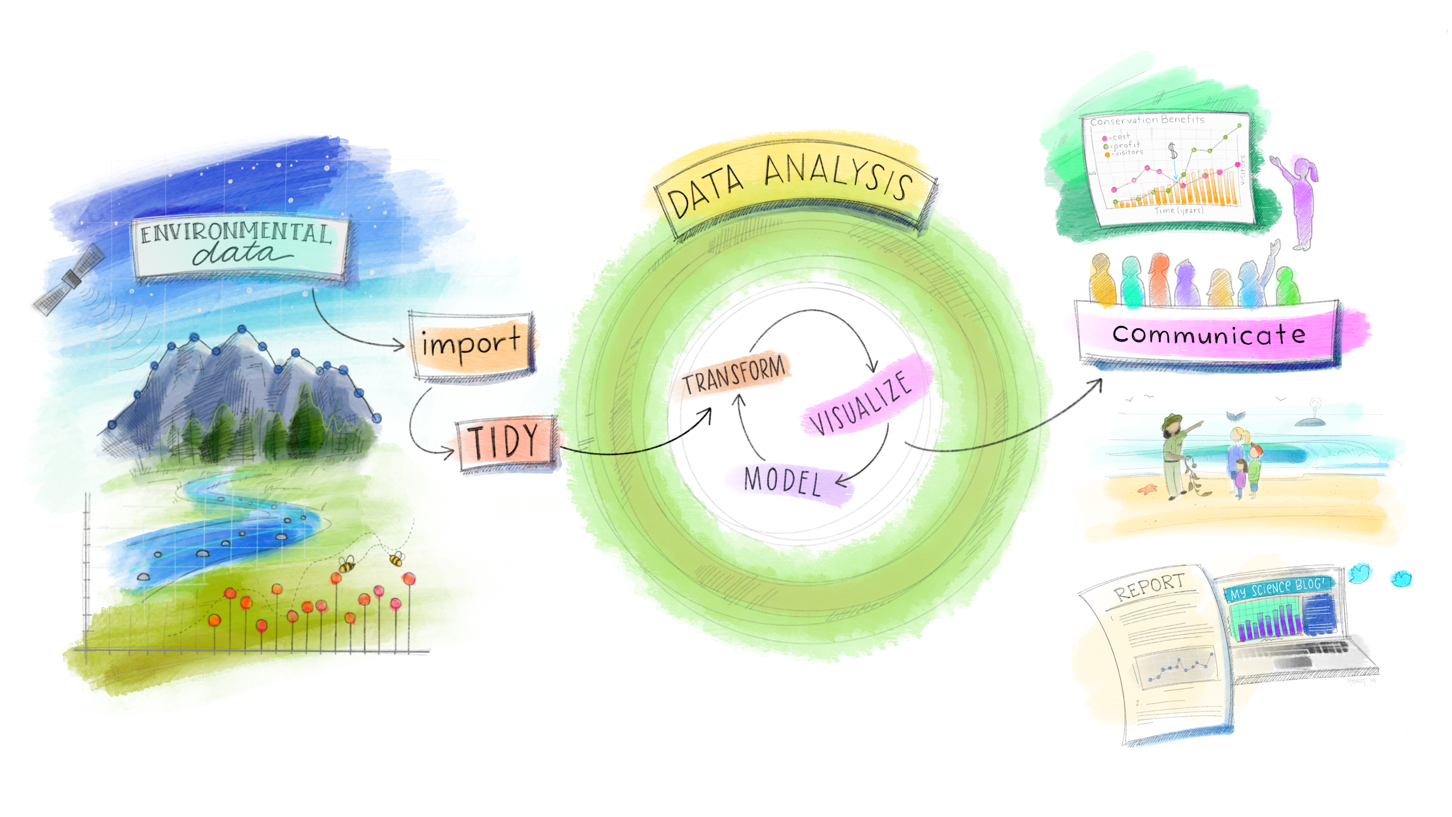
Our Data Science Model
Load packages
This is a critical task:
Every time you open a new R session you will need to load the packages.
Failing to do so will incur in the most common errors among beginners (e.g., ” could not find function ‘x’ ” or “object ‘y’ not found”).
So please always remember to load your packages by running the
libraryfunction for each package you will use in that specific session 🤝
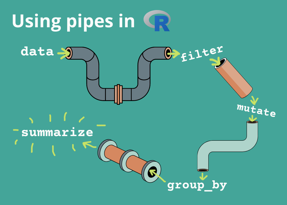
Manipulations on Steroids aka the Pipes’ World!
Pipes are probably the biggest reason why you should use tidyverse for manipulations. Before we learn how to use them please keep in mind that are two types of pipes:
- The magrittr pipe
%>%that comes from themagrittrpackage. Packages in the tidyverse load%>%for you automatically, so you don’t usually load magrittr explicitly. While magrittr pipe was used for a while in the tidyverse world, it is now losing its traction. - In fact, the native pipe
|>is becoming more popular and it is most commonly used.
For this course we will use only the native pipe |>. While for simple cases, |> and %>% behave identically only the native pipe is part of base R, and so it’s always available for you to use. Moreover, |> is simpler than %>% and it works better and faster with more advanced tasks.
You can add the native pipe to your code by using the built-in keyboard shortcut Ctrl/Cmd + Shift + M.
Combining multiple operations with the pipe
Imagine that we want to explore the relationship between the distance and average delay for each destination. There are three steps to prepare our original flights data:
Group flights by destination.
summarize to compute average distance, average delay, and number of flights.
Filter to remove noisy points (less than 20 observations, small sample) and Honolulu airport (almost twice as far away as the next closest airport).
If we put in practice what we learned so far, this code is a little frustrating to write because we have to give each intermediate data frame a name, even though we don’t care about it. Naming things is hard, so this slows down our analysis.
Notice how many assignments and objects (3) I needed to create to get to the desired object. There’s another, much simpler and efficient, way to tackle the same problem thanks to the pipe operator, |>, because we can combine manipulations together:
Notice how many assignments and object (1) I needed to get the desired object, two less than the previous code.
What is great about using pipe is that your code now focuses on the transformations, and not anymore on what’s being transformed, which makes the code easier to read.
In fact, the best way to read the above code is to take each line before the pipe as an imperative statement (remember that the dataset is always the starting point).
Take the flights dataset, then
Group it by destination, then
Summarize it (I want the number of flights at each destination, the average distance and the average delay of each destination), then
Filter the results and include only those destinations with more than 20 flights and exclude Honululu.
As suggested by this reading, a good way to pronounce |> when reading code is “then”. So, remember that you can use the pipe to rewrite multiple operations in a way that you can read left-to-right, top-to-bottom. We’ll use piping from now on because it considerably improves the readability of code and it makes your code more efficient. Working with the pipe is one of the key criteria for belonging to the tidyverse world!
By the way we can use the pipe also to what we have already learned ;-)
Activity 1 You MUST use the pipe to complete the tasks below - 7 minutes
[Write code just below each instruction; finally use MS Teams R - Forum channel for help on the in class activities/homework or if you have other questions]
Keep only the flights in February with more than 75 minutes delay (arrival or departure)
Reorder flights by air_time from bigger to smaller
Keep all columns but those that contain the word “dep”
Create a column named “loss” equal to the difference between arrival delay and departure delay. Make sure to display only the new computed column.
Calculate the median of the distance variable
Missing values
Now it is time to provide an explanation on the na.rm argument that we used in the summarize function. Let’s try one more time in not using it. What happens if we don’t have it?
We get a lot of NAs!

That’s because aggregation functions obey the usual rule of missing values: if there’s any missing value in the input, the output will be a missing value. Fortunately, all aggregation functions have an na.rm argument which removes the missing values prior to computation:
In this case, let’s assume that missing values represent cancelled flights. So, we could also tackle the problem by first removing all the cancelled flights. By doing so we get rid of all missing values and so of the need of using the na.rm argument.
We assigned the above filter to an object so that we can use this dataset in the future. For example, in the below code we don’t need na.rm since we don’t have NAs anymore.
Why producing counts matters?
It is also extremely important that you keep in mind that whenever you do any aggregation, it’s always a good idea to include either a count (n()), or a count of non-missing values (sum(!is.na(x))). That way you can check that you’re not drawing conclusions based on very small amounts of data. Results and conclusions based on few observations contain noise and are drawn based on a small number of events and can lead to incorrect insights.

Caution
Imaginary Scenario: Let’s talk about flight delays and why we can’t always compare them from different times like before, during, and after the pandemic. Things change, and comparisons might not be fair.
Imagine a new direct flight from DeKalb to Potenza. On its first trip, something rare happens: a passenger gets sick, and because of a new rule, the flight is delayed for 14 hours while they wait for a health check.
If we only look at this one flight, we might think the average delay for this route is 14 hours. But that’s not true, it’s just one unusual case. We can’t say all flights on this route are always delayed like this based on one incident. We need more flights to make a fair judgment. If after many flights the delay is still long, then we might think it’s a bad route. But for now, it’s too early to decide based on just one flight.
I hope the scenario made the point on the importance of count clear. Now let’s use a real data example and let’s look at the planes (identified by their tail number) that have the highest average delays:
If you have no info about how many flights each tailnum (airplane) has made. Which one seems the most problematic?
Now you also know how many flights your average is based on. You don’t want to base any conclusion on a small number of observations.
Recap of the summary functions
Just using means and counts can get you a long way, but R provides many other useful summary functions that should be taken in consideration when producing descriptive statistics tables. Here is a list of the most useful ones (make sure to practice them in the activity below):
- Measures of location:
mean(x)andmedian(x). The mean is the sum divided by the length; the median is a value where 50% of x is above it, and 50% is below it.
- Measures of spread:
sd(x). The root mean squared deviation, or standard deviation sd(x), is a standard measure of spread.
- Measures of rank:
min(x)andmax(x). The min will help you identify the smallest value, while the max allows you to find the largest value in column.
Activity 2: Summary functions. Use the pipe to complete the below tasks - 5 minutes:
[Write code just below each instruction; finally use MS Teams R - Forum channel for help on the in class activities/homework or if you have other questions]
Compute the median of the dep_delay variable per each dest? Show also how many flights landed at each destination.
Compute the average air_time variable per each origin? Sort the data by the largest to the smallest average air_time.
Find the max of the arr_delay variable for each month? Show also how many flights you have in each month.
Find the sd of the arr_delay variable for each destination? Sort the data by the smallest to the largest sd.
Creating Full Descriptive Statistic Tables
Now that we went over those functions we need to learn how to use them together to create descriptive/summary statistics tables.

Example 1: Create a descriptive statistic tables that shows min, average, median, max and standard deviation of the arr_delay
Example 2: Create a descriptive statistic tables that shows min, average, median, max and standard deviation of the arr_delay per each carrier. Show also the number of flights operated by each airline.
Example 3: Create a descriptive statistic tables that shows min, average, median, max and standard deviation of the arr_delay per each month. Show also the number of flights departed in each month
Activity 3: Descriptive Statistics Tables. Use the pipe to complete the below tasks - 5 minutes
[Write code just below each instruction; finally use MS Teams R - Forum channel for help on the in class activities/homework or if you have other questions]
Compute a full descriptive stats table of the distance variable per each tailnum?
Compute a full descriptive stats table of the dep_delay variable per each carrier?
Compute a full descriptive stats table of the distance variable per each destination?
Compute a full descriptive stats table of the dep_delay variable per each origin?
Homework 1
[Write code just below each instruction; finally use MS Teams R - Forum channel for help on the in class activities/homework or if you have other questions]
Use the flights dataset and apply the following manipulations at the same time using pipes and do not create any intermediate objects (one big chunk of code):
Make sure your dataset has only the following columns:
month,day,dep_delay,arr_delay,dest,distance,carrierandair_timeReorder your data and show them from the largest
arr_delayflight to the smallest one.Create a column named “distance_km” that is equal to
distance/1.6Per each
carriercompute the “avg_arr_delay”, “min_arr_delay”, “max_arr_delay”, “sd_arr_delay”, “median_arr_delay” and the number of flights operated by eachcarrier.Keep in the output only the 5 carriers with the lowest “median_arr_delay”
Homework 2
[Write code just below each instruction; finally use MS Teams R - Forum channel for help on the in class activities/homework or if you have other questions]
Use the flights dataset and apply the following manipulations at the same time using pipes and do not create any intermediate objects (one big chunk of code):
Keep only flights departed from JFK in February
Make sure your dataset has only the following columns: day, dep_delay, arr_delay, dest,and carrier
Create a column named final_delay that is equal to arr_delay- dep_delay
Per each dest compute the avg_final_delay, min_final_delay, max_final_delay, sd_final_delay, median_final_delay and the number of flights landed there.
Reorder your data and show them from the highest median_final_delay to the smallest one.
When not to use the pipe
Caution
The pipe operator is a powerful tool, but it’s not the only tool at your disposal, and it doesn’t solve every problem! Pipes are most useful for rewriting a fairly short linear sequence of operations. I think you should reach for another tool when:
Your pipes are longer than (say) ten steps. In that case, create intermediate objects with meaningful names. That will make debugging easier, because you can more easily check the intermediate results, and it makes it easier to understand your code, because the variable names can help communicate intent.
You have multiple inputs or outputs. If there isn’t one primary object being transformed, but two or more objects being combined together, don’t use the pipe.
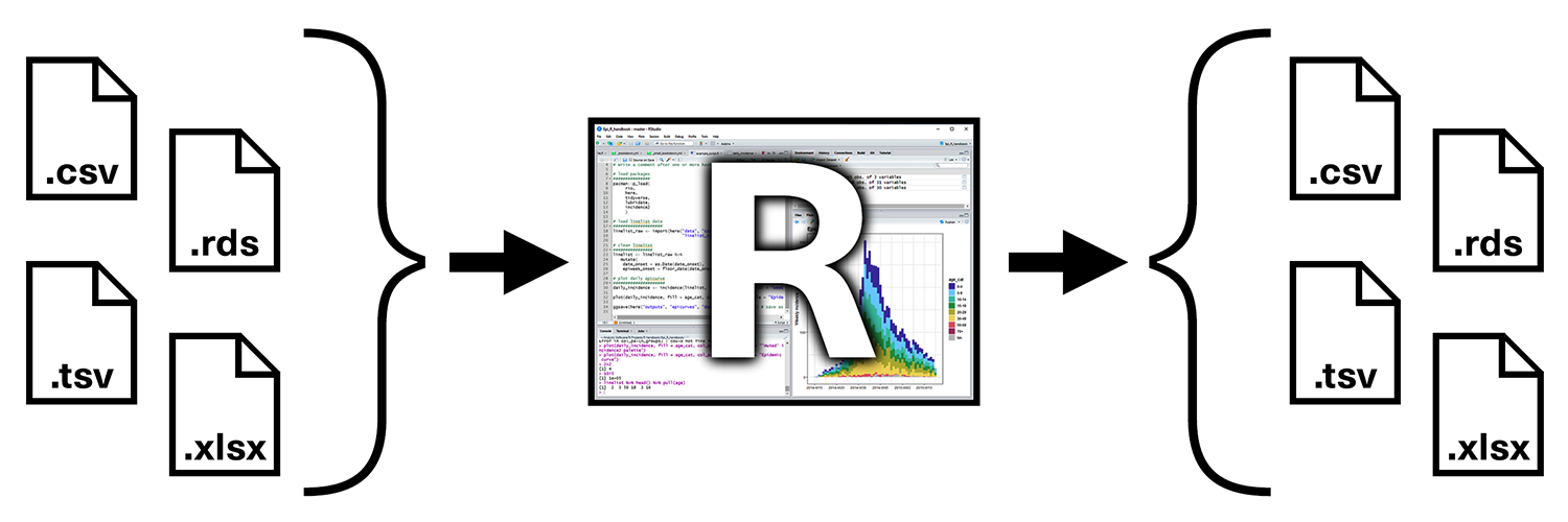
Importing and Exporting data [Skip for now if needed]
Up to this point we have used data available in R packages. We have learned that by loading the packages the datasets are available to us. However, what can we do when the data are not part of R packages? or when we want to bring data outside of R? We need to learn how to import and export data.
Importing data
To load flat files in R we will use the readr package, which is part of the core tidyverse package. Most of readr’s functions are concerned with turning flat files into dataframes (e.g, csv files but similar functions exist also for Excel files or other delimited files). These functions all have similar syntax: once you’ve mastered one, you can use the others with ease. In this course we’ll focus on read_csv(). Not only are csv files one of the most common forms of data storage, but once you understand read_csv(), you can easily apply your knowledge to all the other functions in readr.
The first argument to read_csv() is the most important: it’s the path to the file to read. If you keep your project files in the same folder, you will not have any troubles to access it:
When you run read_csv() it prints out a column specification that gives the name and type of each column. read_csv() uses the first line of the data for the column names, which is a very common convention. The data might not have column names. You can use col_names = FALSE to tell read_csv() not to treat the first row as headings, and instead label them sequentially from X1 to Xn.
Moreover, the read_csv() function will guess the data type of each column by looking at the first 1000 rows. It is your responsibility to make sure that the columns type are correct.
To get other types of data into R, I recommend starting with the tidyverse packages listed below:
havenpackage: reads SPSS, Stata, and SAS files.readxlpackage: reads excel files (both .xls and .xlsx).DBIpackage: along with a database specific backend (e.g. RMySQL, RSQLite, RPostgreSQL etc) allows you to run SQL queries against a database and return a data frame.
Exporting data
Now that we have seen how to bring data into R, what about exporting data from R? The readr package comes also with useful functions for writing data back to disk: e.g., write_csv(). If you want to export to an Excel, use write_excel_csv(). The most important arguments are x (the data frame to save), and path (the location to save it).
Note
Please note that R is running in your web environment, so you might not be able to see the saved file but this functions is very handy when you are collaborating with people not as skilled as you in manipulating data. In fact, after running the code that file will be available in your working directory (which should be your project folder when you run R & RStudio on your computer).